TL;DR — Latent Dirichlet Allocation (LDA, sometimes LDirA/LDiA) is one of the most popular and interpretable generative models for finding topics in text data. I’ve provided an example notebook based on web-scraped job description data. Although running LDA on a canonical dataset like 20Newsgroups would’ve provided clearer topics , it’s important to witness how difficult topic identification can be “in the wild”, and how you might not actually find clear topics — with unsupervised learning, you are never guaranteed to find an answer!

• Acknowledgement: the greatest aid to my understanding was Louis Serrano’s two videos on LDA (2020). A lot of the intuition section is based on his explanation, and I would urge you to visit his video for a more thorough dissection.

Fig 1.0 — the LDA “machine” producing documents

Contents:

Intuition

Maths

Implementation and visualisation

Intuition

Let’s say that you have a collection of different news articles (your corpus of documents), and you suspect that there are several topics that come up frequently within said corpus — your goal is to find out what they are! To get there you make a few key assumptions:

• The distributional hypothesis: Words that appear together frequently are likely to be close in meaning;
• each topic is a mixture of different words (Fig 1.1);
• each document is a mixture of different topics (Fig 1.2).

Fig 1.1 — Topics as a mixture of words

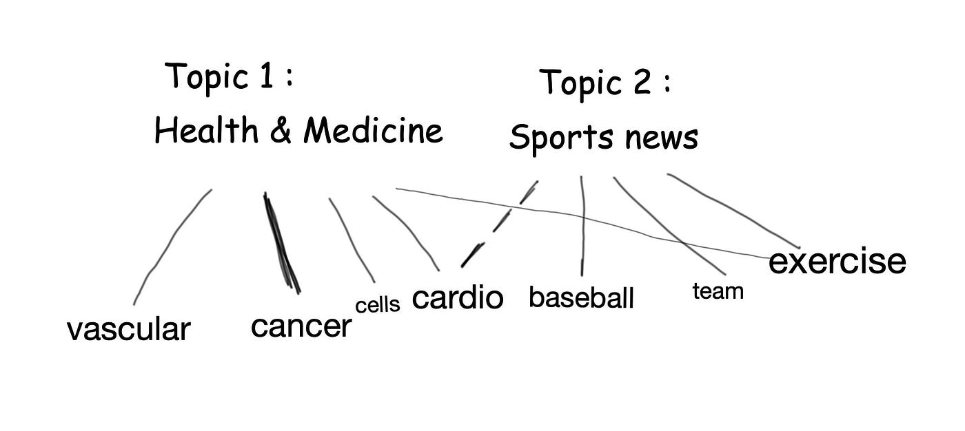
In Fig 1.1 you’ll notice that the topic “Health & Medicine” has various words associated with it to varying degrees (“cancer” is more strongly associated than “vascular” or “exercise”). Note that different words can be associated with different topics, as with the word “cardio”.

Fig 1.2 — Document as a mixture of topics

In Fig 1.2 you’ll see that a single document can pertain to multiple topics (as colour-coded on the left). Words like “injury” and “recovery” might also belong to multiple topics (hence why I’ve coloured them in more than one colour).

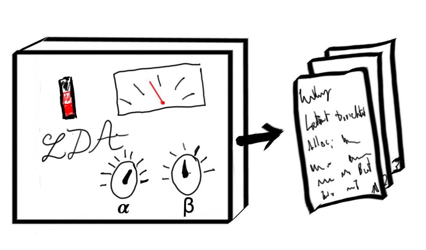
Now LDA is a generative model — it tries to determine the underlying mechanism that generates the articles and the topics. Think of it as if there’s a machine with particular settings that spits out articles, but we can’t see the machine’s settings, only what it produces. LDA creates a set of machines with different settings and selects the one that gives the best-fitting results (Serrano, 2020). Once the best one is found, we take a look at its “settings” and we deduce the topics from that.

So what are these settings?

First, we have something called the Dirichlet (pronounced like dee-reesh-lay) prior of the topics. This is a number that says how sparse or how mixed up our topics are. In L Serrano’s video (which I highly recommend!) he illustrates how visually you can think of this as a triangle (Fig 1.3) where the dots represent the documents and their position with respect to the corners (i.e. the topics) represents the how they’re related to each of the topics (2020). So a dot that is very close to the “Sports” vertex will be almost entirely about sport.

Fig 1.3 — Dirichlet distribution of topics

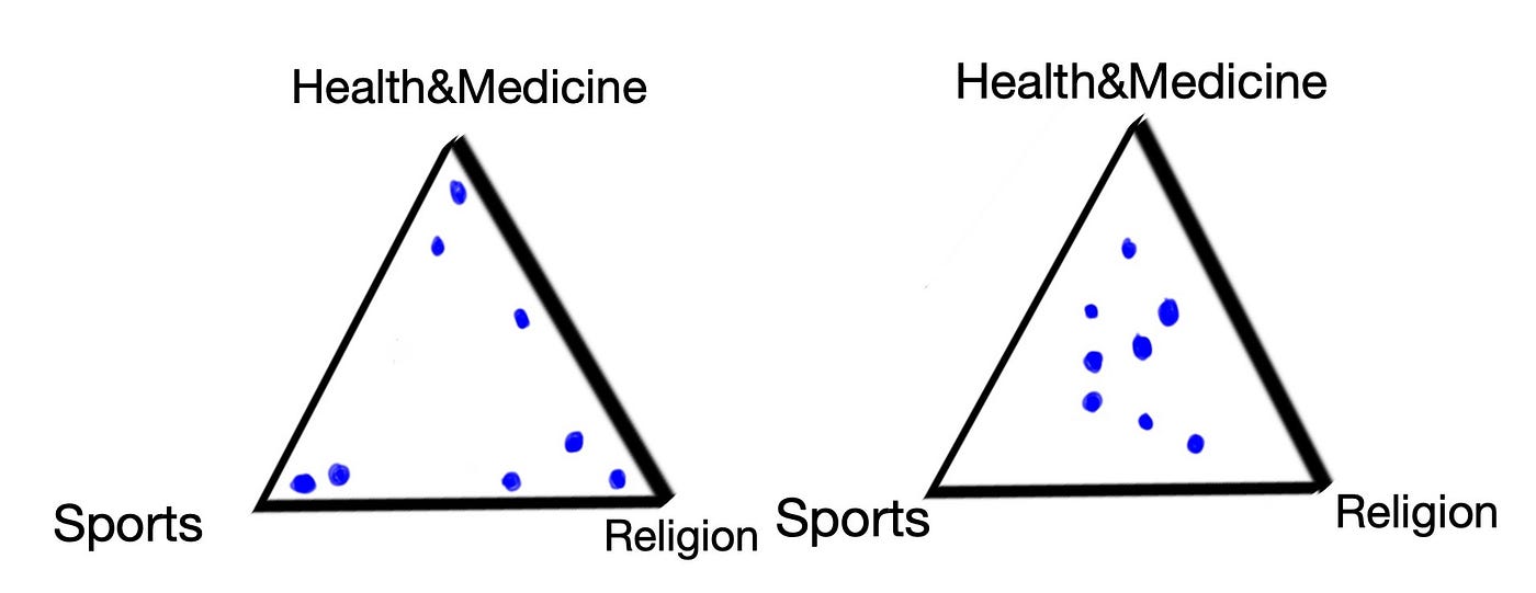
In the lefthand triangle the documents are fairly separated, most of them neatly tucked into their corners (this corresponds to a low Dirichlet prior, alpha<1); on the right they are in the middle and represent a more even mix of topics (a higher Dirichlet prior, alpha>1). Look at the document in Fig 1.2 and, given the mix of topics, have a think about where you think it would be placed in the triangle on the right (my answer is that it’d be the dot just above the one closest to the Sports corner).

Second, we have the Dirichlet prior of the terms (all the words in our vocabulary). This number (whose name is beta) has almost exactly the same function as alpha — except that it determines how the topics are distributed amongst the terms.

Fig 1.4 Dirichlet distribution of terms; the numbers are proportional to how much each word is associated with each respective topic

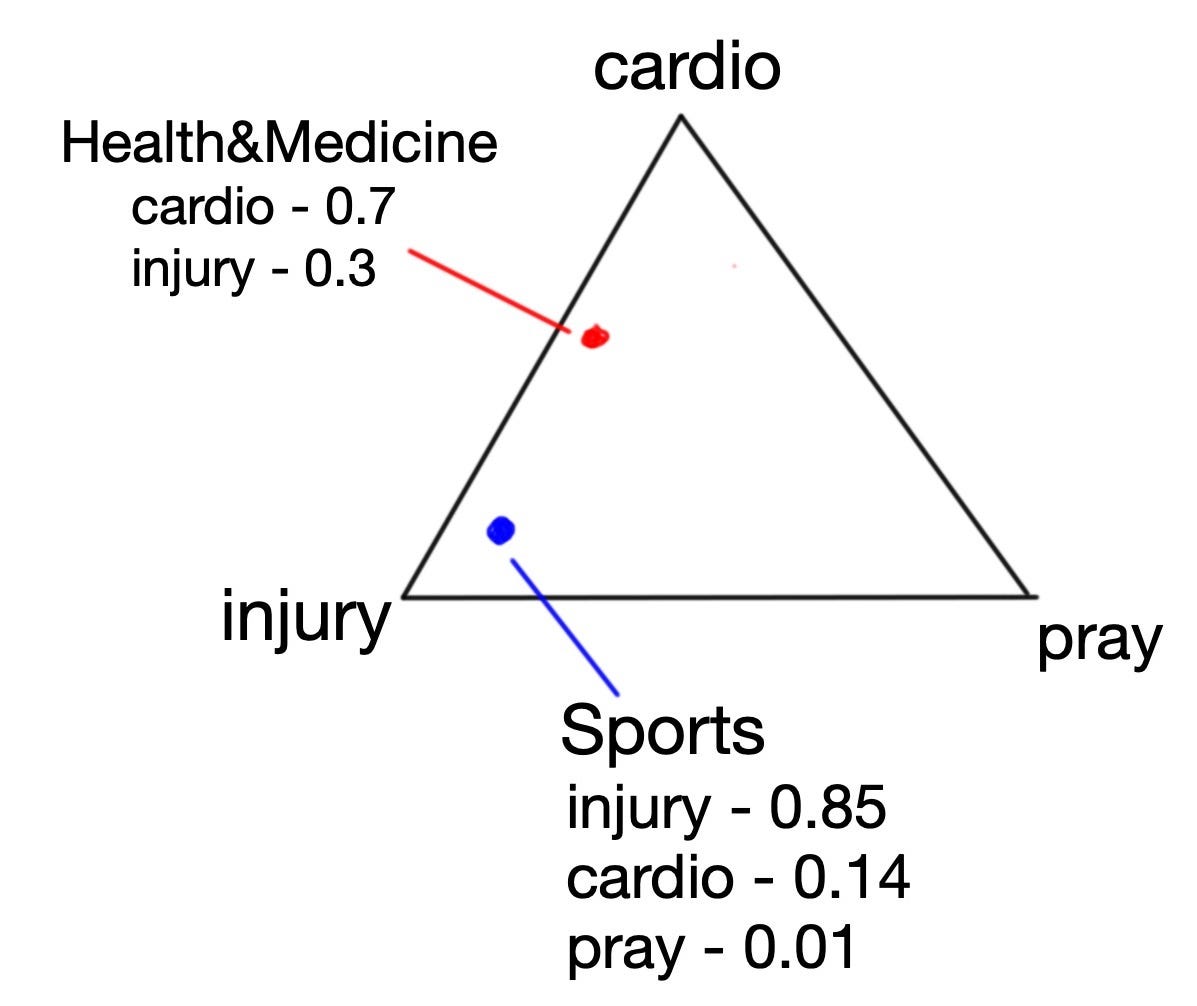
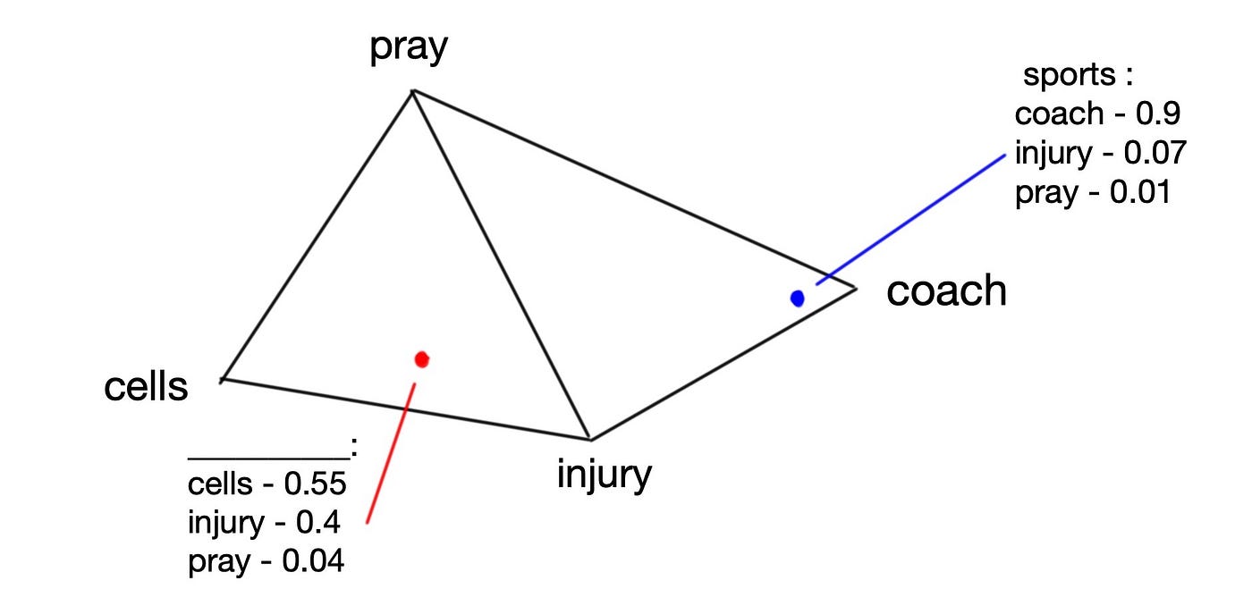
As we said before, the topics are assumed to be mixtures (more precisely, distributions) of different terms. In Fig 1.4 “Sports” is mostly drawn towards “injury”. “Health&Medicine” is torn between “cardio” and “injury” and has no association with the term “pray”.

But wait, our vocabulary doesn’t consist of just 3 words! You’re right! We could have a vocabulary of 4 words (as shown in Fig 1.5)! Trouble is that visualising a typical vocabulary of N words (where N could be 10'000) would require a generalised version of the triangle shape, but in N — 1 dimensions (the term for this is an n-1 simplex). This is where the visuals stop and we trust that the maths of higher dimensions will function as expected. This also applies to the topics — very often we’ll find ourselves with more than 3 topics.

Fig 1.5 — which topic is the red one, based on the distribution of terms?

An important clarification: in LDA we start with values of alpha and beta as hyperparameters, but these numbers only tell us whether our dots (documents / topics) are generally concentrated in the middle of their triangles or closer to the corners. The actual positions within the triangle (simplex) are guessed by the machine — the guesswork is not random, it’s heavily weighted by the Dirichlet priors.

So the machine creates the two Dirichlet distributions, distributes the documents and topics on them and then generates documents based on those distributions (Fig 1.6). So, how does the last step happen, the generation part?

Fig 1.6 — the LDA “machine” producing documents

Remember at the start we said that topics are seen as mixtures / distributions of words and documents as mixtures / distributions of topics? Going from left to right in Figure 1.7 we start with a document, somewhere in the triangle, torn between our 3 topics. If it’s near the “Sports” corner, this means that the document will be mostly about Sports, with some mentions of “Religion” and “Health&Medicine”. So we know the topic composition of the document → therefore we can estimate what words will come up. We will be sampling (i.e. randomly pulling out) words mostly from Sports, some from Health&Medicine and a very small amount from Religion (Fig 1.7). Here’s a question for you: looking at the triangle at the bottom of Fig 1.7, do you think word 2 will come up or not?

Fig 1.7 — how the two Dirichlet distributions feed into our document generation

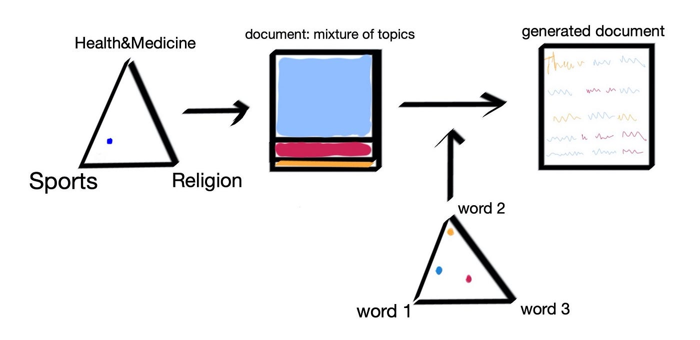
The answer is that it might: remember that topics are mixtures of words. You might be thinking that word 2 is very strongly related to the yellow (Religion) topic, and since this topic is very sparse in this document word 2 won’t come up as much. But remember that a. word 2 is also associated with the blue, Sports topic and b. the words are sample probabilistically, so every word has some non-zero chance of appearing.

The words in our final, generated document (on the right end of Fig 1.7) will be compared to the words in the original documents. We won’t get the same document, BUT when we compare a range of different LDA “machines” with a range of different distributions, we find that one of them was closer to generating the document than the others were and that’s the LDA model that we choose.

Maths

A normal statistical language model assumes that you can generate a document by sampling from a probability distribution over words, i.e. for each word in our vocabulary there is an associated probability of that word appearing.

LDA adds a layer of complexity over this arrangement. It assumes a list of topics, k. Each document m is a probability distribution over these k topics, and each topic is a probability distribution over all the different terms in our vocabulary V. That is to say that each word has various probabilities of appearing in each topic.

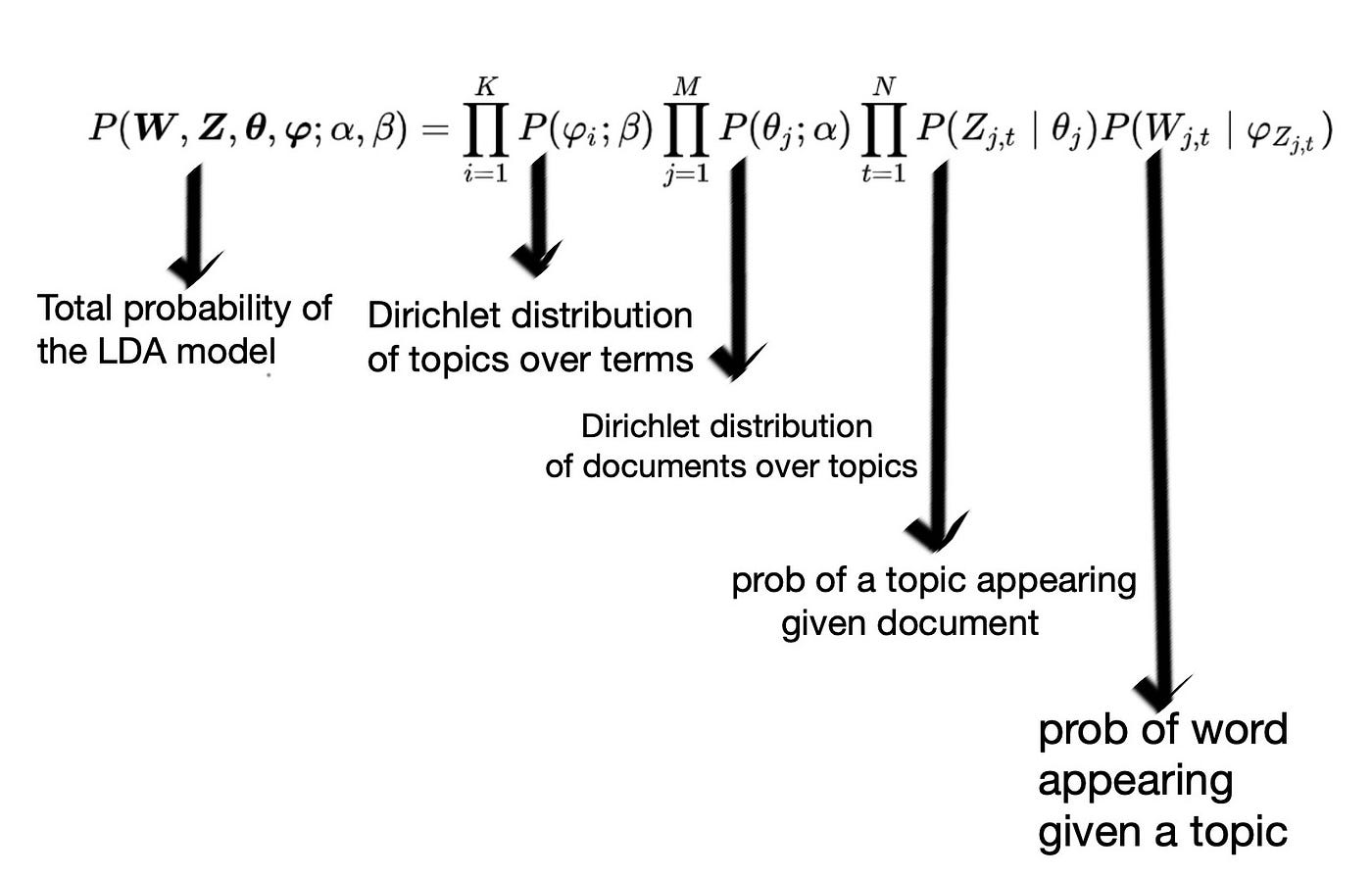
The full probability formula that generates a document is in Figure 2.0 below. If we break this down, on the right hand side we have three product sums:

• Dirichlet distribution of topics over terms: (corresponds to Fig 1.4 and 1.5) for each topic i amongst K topics, what is the probability distribution of words for i.
• Dirichlet distribution of documents over topics: (corresponds to Fig 1.3) for each document j in our corpus of size M, what is the probability distribution of topics for j.
• Probability of a topic appearing given a document X the probability of a word appearing given a topic: (corresponding to the two rectangles in Fig 1.7) how likely is it that certain topics, Z, appear in this document and then how likely is that certain words, W, appear given those topics.

Fig 2.0 — LDA formula

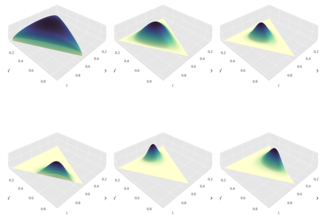
The first two sums contain symmetric Dirichlet distributions which are prior probability distributions for our documents and our topics (Fig 2.1 shows a set of general Dirichlet distributions, including symmetric ones).

Fig 2.1 — By Empetrisor — Own work, CC BY-SA 4.0, https://commons.wikimedia.org/w/index.php?curid=49908662

The 3rd sum contains two multinomial distributions, one over topics and one over words — i.e. we sample topics from a probability distribution of them and then for each topic instance we sample words from a probability distribution of words for that particular topic.

As was mentioned at the end of the Intuition section, using the final probability we try to generate the same distribution of words as the one that we get in our original documents. The probability of achieving this is very, very low, but for some values of alpha and beta the probability will be less low.

Interpreting an LDA model and its topics

What metrics do we use for finding our latent topics? As Shirley and Sievert note:

“To interpret a topic, one typically examines a ranked list of the most probable terms in that topic, […]. The problem with interpreting topics this way is that common terms in the corpus often appear near the top of such lists for multiple topics, making it hard to differentiate the meanings of these topics.” (2014)

That is exactly the problem we’ve stumbled into in the next section, Implementation. Therefore we use an alternative metric for interpreting our topics — relevance (Shirley and Sievert, 2014).

Relevance

This is an adjustable metric that balances a term’s frequency in a particular topic against the term’s frequency across the whole corpus of documents.

In other words, if we have a term that’s quite popular in a topic, relevance allows us to gauge how much of its popularity is due to it being very specific to that topic and how much of it is due to it just being a work that appears everywhere. An example of the latter would be “learning” in the job description data. When we adjust relevance with a lower lambda (i.e. penalising terms that just happen to be frequent across all topics), we see that “learning” is not that special a term, and it only comes up frequently because of its prevalence across the corpus.

The mathematical definition of relevance is:

• r — relevance
• ⍵ — a term in our vocabulary
• k — a topic amongst the ones our LDA has produced
• λ — the adjustable weight parameter
• 𝝓kw — probability of a term appearing in a particular topic
• pw — the probability of a term appearing inside the corpus as a whole

Apart from lambda, λ, all the terms are derived from the LDA data and model. We adjust lambda in the next section to help us derive more useful insights. The original paper authors kept lambda in the range of 0.3 to 0.6 (Shirley and Sievert, 2014).

Implementation and visualisation

The implementation of sklearn’s LatentDirichletAllocation model follows the pattern of most sklearn models. In my notebook, I:

1. Pre-processed my text data,
2. Vectorised it (resulting in a document-term matrix),
3. Fit_transformed it using LDA and then
4. Inspected the results to see if there are any emergent, identifiable topics.

The last part is highly subjective (remember this is unsupervised learning) and is not guaranteed to reveal anything really interesting. Furthermore the ability to identify topics (like clusters) depends on your domain knowledge of the data. I recommend also altering the alpha and beta parameters to match your expectations of the text data.

The data I’m using is job post description data from indeed.co.uk. The dataframe has many other attributes than text, including whether I used the search terms “data scientist”, “data analyst” or “machine learning engineer”. Can we find some of the original search categories in our LDA topics?

In the gist below you’ll see that I’ve vectorised my data and passed it to an LDA model (this happens under the hood of the data_to_lda function).

Running this code and the print_topics function will produce something like this:

Topics found via LDA on Count Vectorised data for ALL categories:  
  
Topic #1:  
software; experience; amazon; learning; opportunity; team; application; business; work; product; engineer; problem; development; technical; make; personal; process; skill; working; science  
  
Topic #2:  
learning; research; experience; science; team; role; work; working; model; skill; deep; please; language; python; nlp; quantitative; technique; candidate; algorithm; researcherTopic #3:  
learning; work; team; time; company; causalens; business; high; platform; exciting; award; day; development; approach; best; holiday; fund; mission; opportunity; problem  
  
Topic #4:  
client; business; team; work; people; opportunity; service; financial; role; value; investment; experience; firm; market; skill; management; make; global; working; support...

The “print_topics” function gives the terms for each topic in decreasing order of probability, which can be informative. It’s at this stage that we can start trying to label the emergent, latent topics from our model. For instance, Topic 1 seems to be related mildly related to ML engineer skills and requirements (the mention of “amazon” relates to using AWS — this is something I found from the EDA stage of the project in another notebook); meanwhile, Topic 4 clearly has a more client-facing or business-oriented theme, given terms like “market”, “financial”, “global”.

Now those two categories might seem a bit far-fetched to you and that’s a fair criticism. You may also have noticed that using this method for topic determination is hard. So, let’s turn to pyLDAvis!

pyLDAvis

Using pyLDAvis, the LDA data (which in our case, was 10-dimensional) has been decomposed via PCA (principal component analysis) to be only 2-dimensional. Thus it has been flattened for the purposes of visualisation. We have ten circles and the center of each circle represents the position of our topic in the latent feature space; the distances between topics illustrates how (dis)similar the topics are and the area of the circles is proportional to how many documents feature each topic.

Below I’ve shown how you insert an already trained sklearn LDA model in pyLDAvis. Thankfully the people responsible for adapting the original LDAvis (which was R model) to python made it communicate efficiently with sklearn.

And in Fig 3.0 is the plot we generate:

Fig 3.0 — pyLDAvis interactive plot

Interpreting pyLDAvis plots

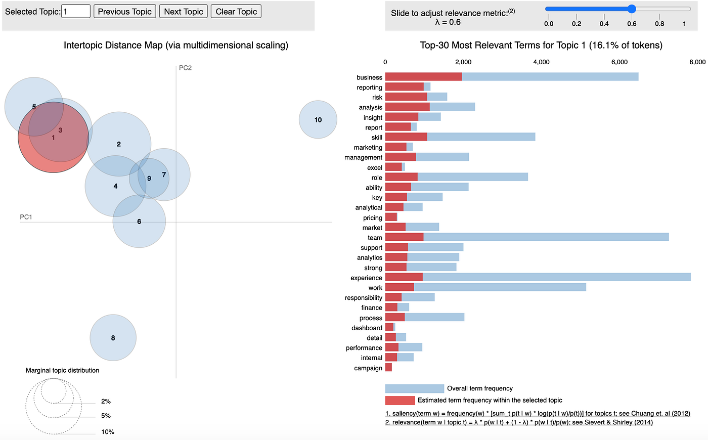
The LDAvis plot comes in two parts — a 2-dimensional ‘flattened’ replotting of our n-dimensional LDA data and an interactive, varying horizontal bar-chart of term distributions. Both of these are shown in Fig A1.0. One important feature to note is that the right-hand bar chart shows the terms in a topic in decreasing order of relevance, but the bars indicate the frequency of the terms. The red section represents the term frequency purely within the particular topic; the red and blue represent the overall term frequency within the corpus of documents.

Adjusting λ (lambda)

If we set λ equal to 1, then our relevance is given purely by the probability of the word to that topic. Setting it to 0 will result in our relevance being dictated by specificity of that word to the topic — this is because the right hand term divides the probability of a term appearing in a particular topic divided by the probability of the word appearing generally — thus, highly frequent words (such as ‘team’, ‘skill’, ‘business’) will be downgraded heavily in relevance when we have a lower λ value.

Fig 3.1 — setting lambda to 1

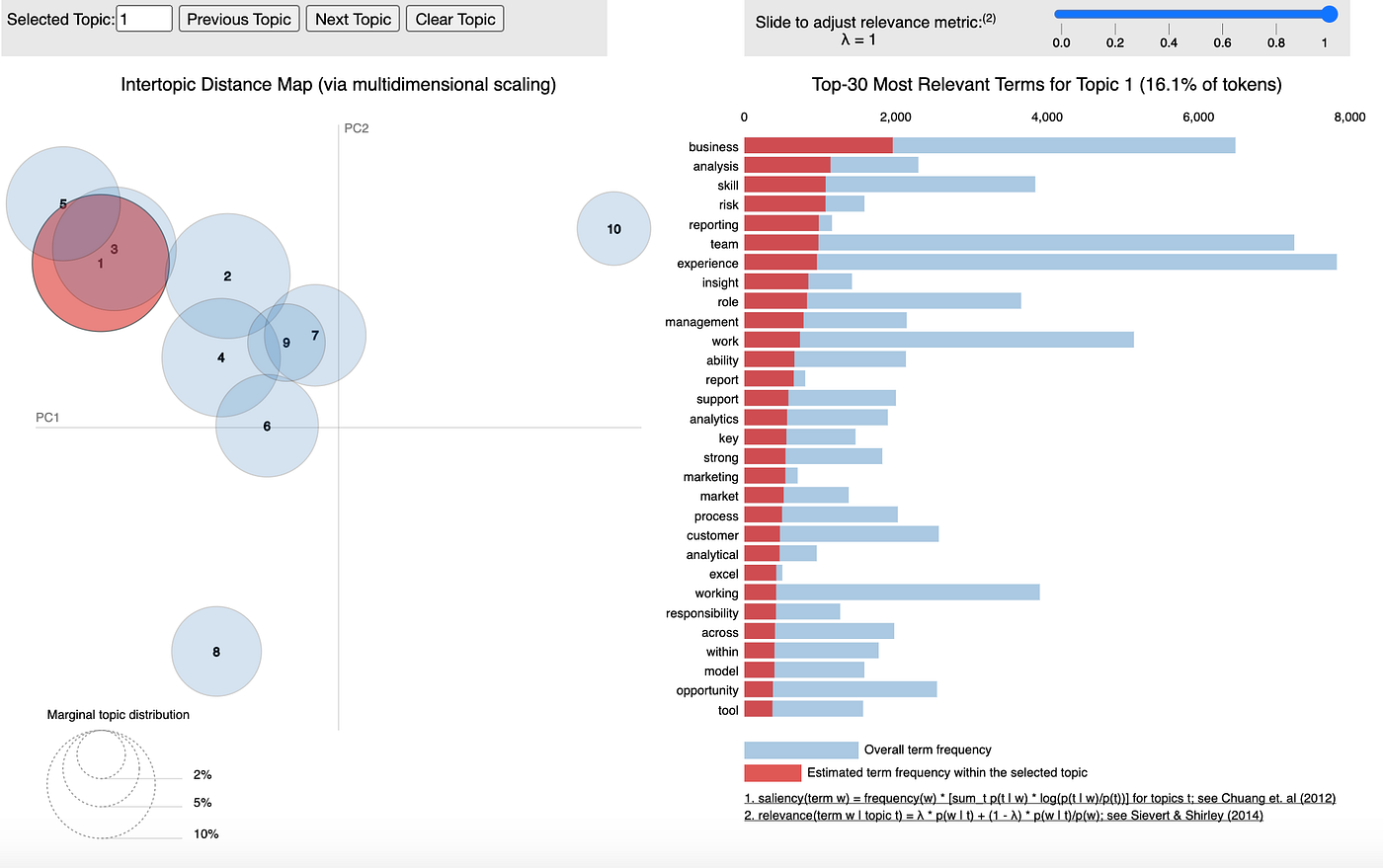
In Fig 3.1 λ was set to 1 and you can see that the terms tend to match the ones that dominate across the board generally (i.e. like in our print-outs of the most popular terms for each topic). This was only done for topic 1, but when I changed topic the distribution of top-30 most relevant terms barely changed at all!

Now, in Fig 3.2 λ was set to 0 and the terms changed completely!

Fig 3.2 — lambda set to 0

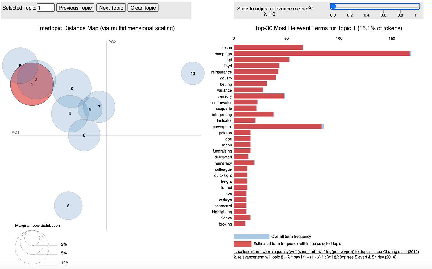
Now we have highly specific terms, but pay attention to the scale at the top — the most relevant word appears about 60 times. That’s quite a come down after over 6000! Also, these words won’t necessarily tell us anything interesting. If you select a different topic with this lambda value you will keep getting junk terms that aren’t necessarily that important.

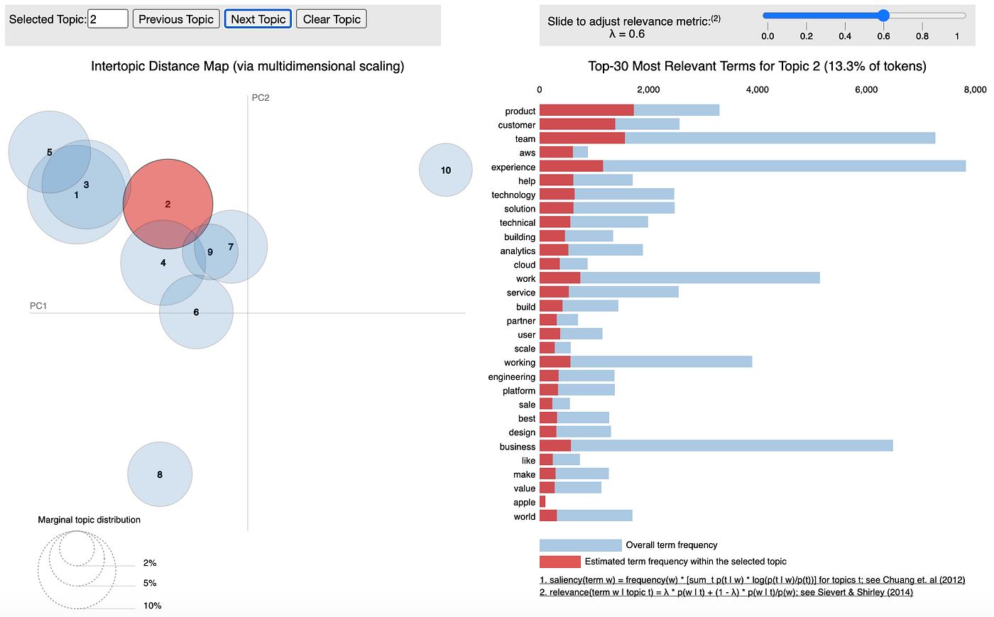
In Fig 3.3 I’ve set lambda to 0.6 and I am exploring topic 2. Right off the bat there is a significant theme here surrounding engineer work, with terms like “aws”, “cloud” and “platform”.

Fig 3.3 — lambda = 0.6

Another great thing that you can do with pyLDAvis is visually inspect the conditional topic distribution given a word, simply by hovering over the word (Fig 3.4). Below we can see just how much “NLP” is split amongst several topics — not a lot! This gives me further reason to believe that topic 6 is focused on NLP and text-based work (terms like “speech”, “language”, “text” also help in that regard). An interesting insight for me is the fact that “research” and “PhD” co-occur so strongly in this topic.

Fig 3.4 — conditional topic distribution for “NLP”

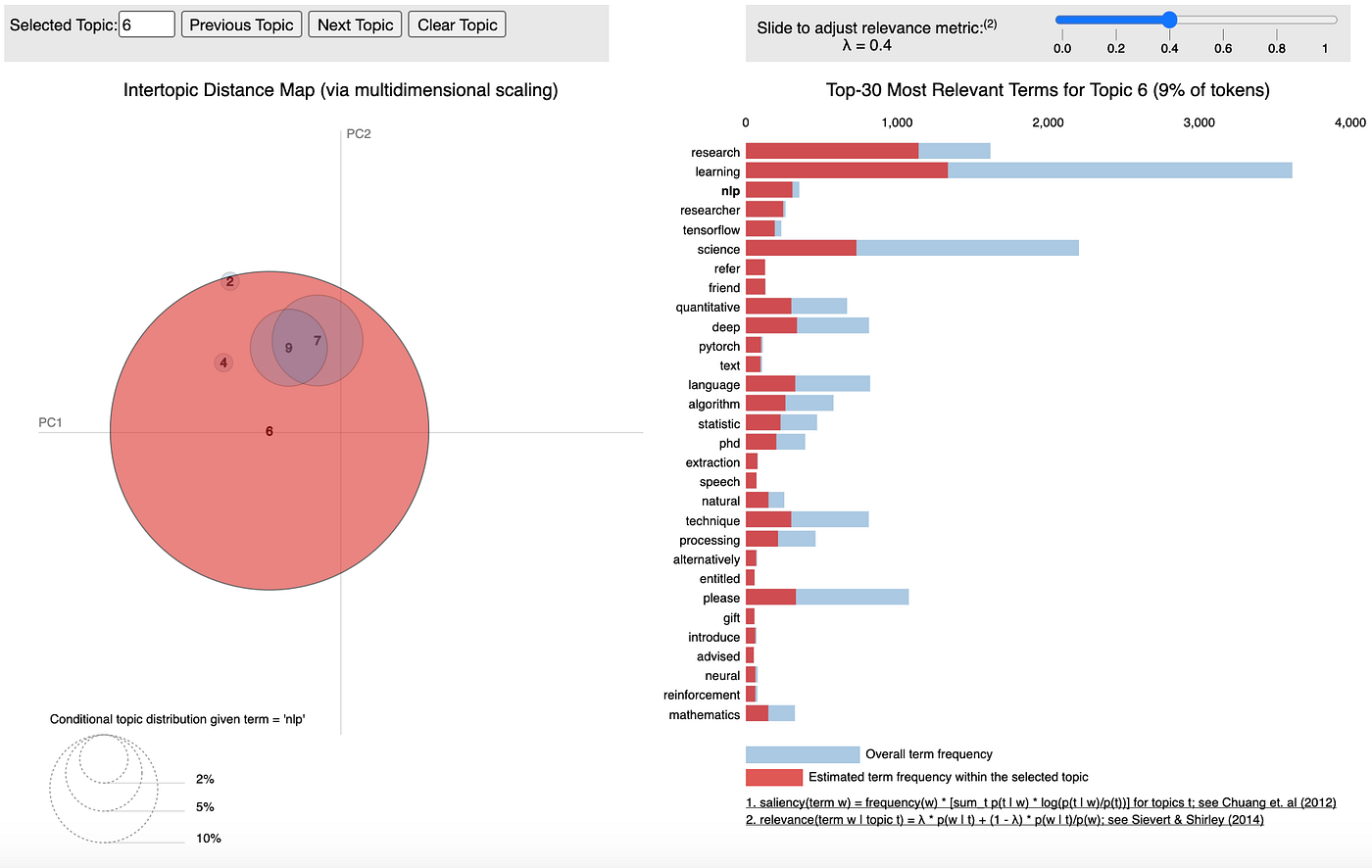
Does this mean that NLP-focussed roles in the industry demand higher education than other roles? Do they demand previous research experience more often than other roles? Are NLP roles perhaps more fixated on experimental techniques and thus require someone with knowledge of the cutting edge?

While the interactive plot generated cannot deliver concrete answers, what it can do is provide us with a starting position for further investigation. If you’re in an organisation where you can run topic modelling, you can use LDA’s latent themes to inform survey-design, A/B testing or even correlate it with other available data to find interesting correlations!

I wish you the best of luck in topic modelling. If you’ve enjoyed this lengthy read, please give me as many claps as you think are appropriate. If you have knowledge of LDA and think I’ve gotten something even partially wrong please leave me a comment (feedback is a gift and all that)!

References

1. Serrano L. (2020). Accessed online: Latent Dirichlet Allocation (Part 1 of 2)
2. Sievert C. and Shirley K (2014). LDAvis: A method for visualizing and interpreting topics. Accessed online: Proceedings of the Workshop on Interactive Language Learning, Visualization, and Interfaces